Capay Canyon Ranch, is a family run almond growing and processing business, located in Yolo County. Fast track learning about [California] agriculture can be found in these CA Grown videos hosted by the CDFA. Explore also these educational episodes from True Food TV e.g. Pecan | How does it Grow?
All posts by cs
Chilling Out
It’s hard to believe but here we are back to the beginning; wash rinse repeat, it’s springtime bloom already. The growing cycle renews. Winter sanitation was completed, and soil moisture adjusted (rainfall was rather weak this go round). The season is off to a start with the early arrival of warm daytime temperatures. This brings on the flowers for pollination and luckily the bee hives have been on site for the last two weeks to take full advantage of the warm afternoons.
Nights can still be cold at this juncture and our Monday and Tuesday forecast frost/freeze is a potential pitfall:
Advection frosts can be severe and usually result in more damage. They occur with wind present as cold air comes from areas outside the orchard. Not happening.
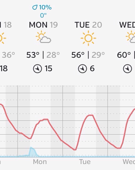
Next weeks scenario is for mild, radiation frost that occurs on still, clear nights, often with the development of a strong inversion.
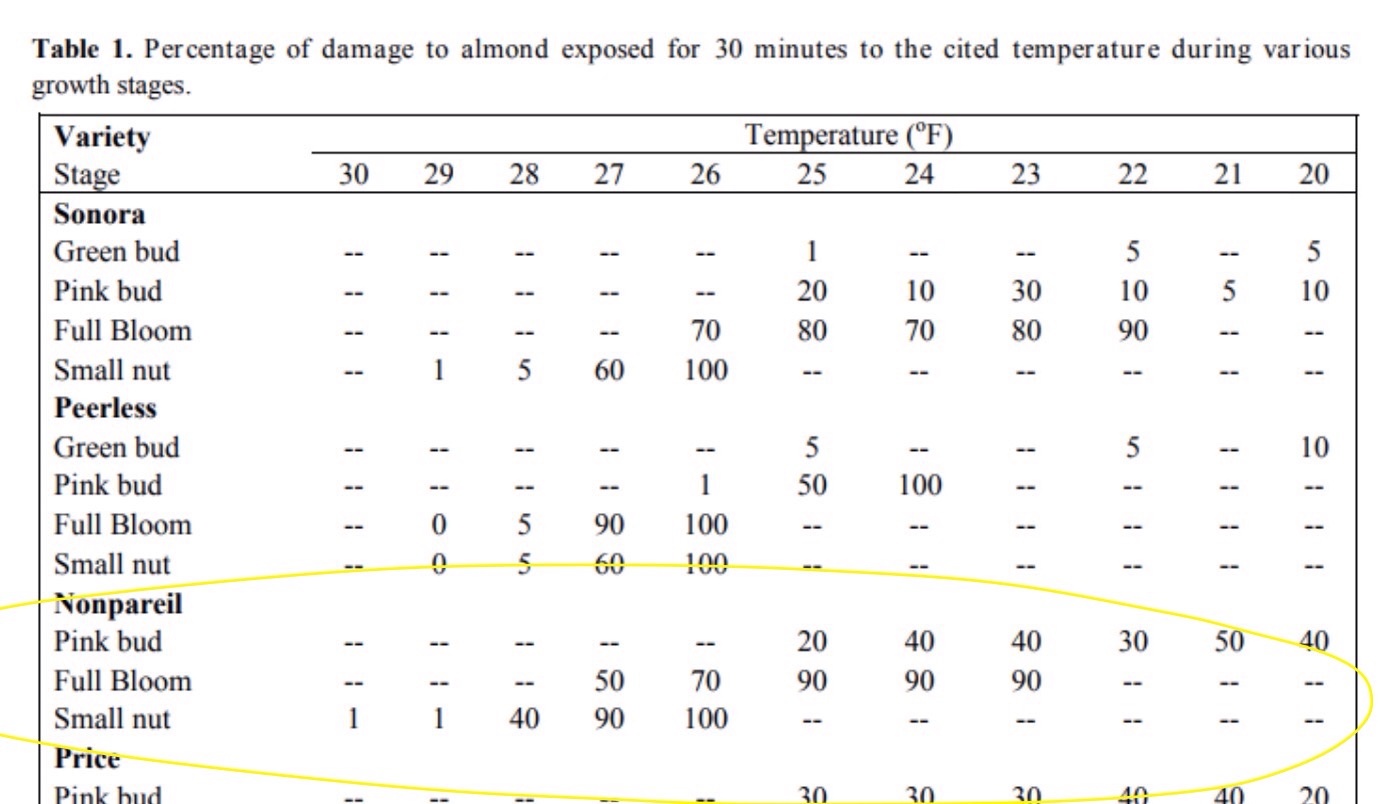
At pink bud, flowers are more resistant to cold compared to full bloom, which is more resistant than at petal fall or with small nuts. The following table is a guideline.
We are not completely at the mercy of Mother Nature:
Groundcover condition affects orchard minimums with any cover taller than 4 inches in height generally being colder. Soil heat storage is reduced because sunlight is reflected and water is evaporated. Keeping groundcovers cut short to 2 inches or less during frost season allows sunlight to reach the soil surface, and increases soil heat storage resulting in a warmer orchard through the night. Bare soil with soil moisture near field [moisture] capacity (about 2 days after wetting) is warmest because it transfers and stores heat best. A light irrigation to moisten dry soil a day or two before a frost will help obtain the greatest heat . Running the system during a frost may provide slight benefits due to radiation heating from the wetted area beneath the trees.  Flood irrigation for frost protection works in a similar fashion but due to larger water volumes it will provide more protection as long as ice doesn’t form on the water’s surface. In our experiments with micro-sprinklers, applying 15, 25, and 40 gallons per minute per acre resulted in little difference in observed air temperatures. However, exposed temperatures were 1 to 2 degrees warmer at the higher water rates. Exposed temperature is what the buds themselves experience. — via UCCE farm advisor and UC Davis biometeorologist http://bluediamondgrowers.com/grower-news/frost-protection/
Our current status is firm, moist earth with no ground cover. We are presently between pink bud and full bloom. A technical malfunction with the drip irrigation system means that a precautionary irrigation will not be possible.
Fortunately, as the chart presentation depicts, we will be alright; it is the early nut stage that is most at risk.
Enemy in the Vineyard
As a percentage of expense (22%), we spend considerable effort in controlling insect pests and weeds on our farm. Invoice statements from a supplier arrive with esoteric names such as Intrepid 2F, Teb 45DF, AbbA Ultra, Luna Experience, Provoke, Deploy… These are chemicals that are broadcast to keep from losing the war. We are doing battle against freeloading critters and pesky weeds that seek to throttle our production yield; if not choke off our margins of gain entirely. It is a challenge to figure out into which manner of classification we must group them. Insecticide, Pesticide, Fungicide, Herbicide?
In the vineyard we are up against hairy fleabane, horsetail, johnsongrass, powdery mildew, leafroller, leafhopper, and spider mites, to name the usual suspects.
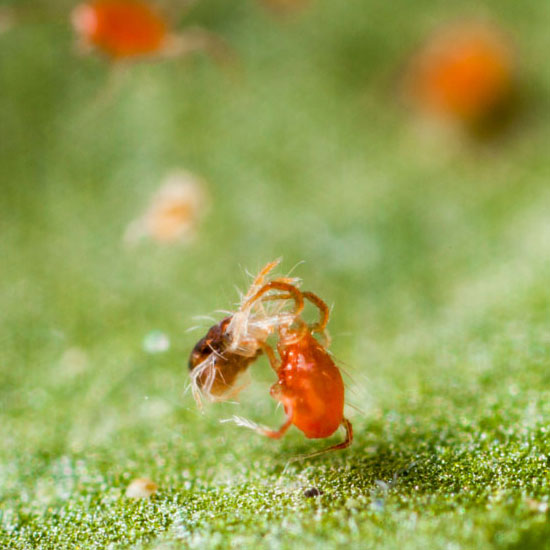
There are other ways to fight. The organic option may become the holy grail at some point. For instance: ladybugs, lacewing and minute pirate bugs, are all voracious predators beneficially consuming the leafhopper larvae and their eggs. Sixspotted thrips are a natural predators of the mites. Organically acceptable methods include biological and cultural control schemes such as oil or soap sprays. Unfortunately, the sure thing – nuke option – with chemicals cannot co-exist with the natural predators. There’s no discrimination between friend or foe.
A third solution? Genetic resistance as cost-effective and environmentally friendly method. However, this would entail the deployment of a new grape variety — not a trivial conversion. Furthermore, our adversaries enately adapt to new environments and challenges. Who’s to say that they or some relation might not evolve to savor the newest iteration.
We already know that deviant pests can become tolerant to the nasty chemicals that we throw at them. In fact, every season we strike with different blended variations to catch them off guard.
And so the struggle goes. Like to join up for the cause? Thirst for learning? Here is a Knowledge Expectations link that outlines what one must command in order to gain the rank of [accredited] Agricultural Pest Control Adviser (PCA).
Giving it Meaning and with Emphasis
Modern Irrigation: We track a handful of metrics. Some of them are constants e.g. the pricing rate of energy. There are data points such as pump operational hours that are logged in tabular form. All of this information can be spun with a spreadsheet yielding useful intel.
Recall a previous post on scientific irrigation? It made reference to how much moisture a plant needs to maximize the photosynthetic process and thus crop harvest yield. Too much water is a waste and not enough is detrimental. The task then is to compute how much water are we putting down.
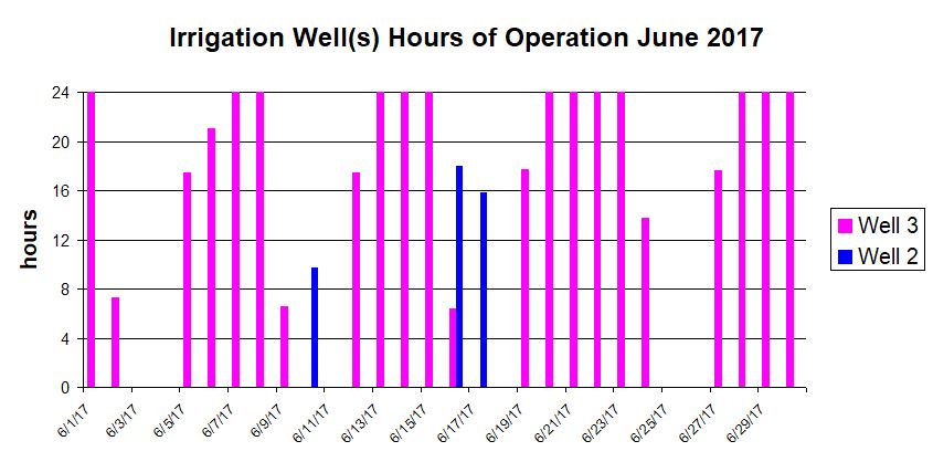
A first thing to understand is the concept of irrigation sets. Each of the vertical bars indicates a set. Think of an irrigator person adjusting or setting the flow so that he can leave for a few hours or attend to other jobs. (He needs to do this precisely because if the flow is too high then flooding occurs) The month of June requires a lot of water. It’s a vigorous growth period. Here you can see that the irrigation set can last for multiple days and extend into a 24hr interval.
Were’d this data come from? In times previous the reporting was scattered and usually furnished in an end of month statement summary. For example the utility company would tell us the energy total for the month and at the end of the period a field hand would read a flowage meter and pass along a reading. Knowing the previous months reading we could find the difference and figure out a total. Bare bones basic and lacking any detail, right? Did I mention that the report dates rarely coincide.
These days, we have smart meters and telemetry that will allow us near real time data collection. A side effect is that the quantity of data can become immense and we’re back to square one trying to make sense of it.
Gathering the data is a first challenge. It comes from scraping an online file and of course it is in a format that doesn’t present in any concise way.
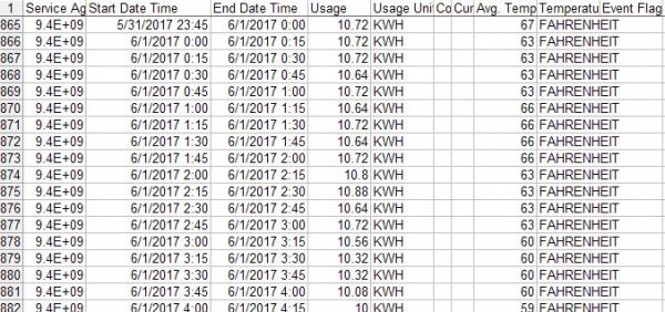
This is just a snippet. It has 3,500 rows and that is just for half the year and only one of the wells! So next step is to fold, spindle or mutilate that raw data to give it meaning.
Observe that each row is a 00 :15 minute window. A daily output however is sufficient granularity. Further we need to convert the energy usage for presentation in layman’s terms. We want to know for how many hours the pump motors ran, on what days, and what proportional share of energy they each used to move “x” amount of water.
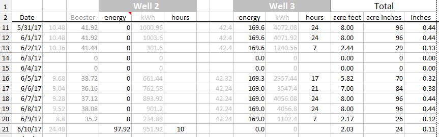
“X” amount of water: As said, the water flow meter is our primary tool but only a monthly itemization. There are some known constants that will break this down into a daily amount. We know the pumping capacity based on recent testing and now that we have the daily usage (above) we can formulate the output. More variables and constants and arithmetic that we use:
- output in GPM is 1,792 and when multiplied by 60 converts to gallons/hour
- 32,585 gallons == 1 acre foot (an old school agricultural unit of measure)
- divide 32,585 by our gallons per hour determines how many hours of pumping
- energy consumption rate expressed in kWh is 169
- multiply hours of pumping times 169 to find energy per acre foot
- cost of energy is $0.19 per kWh
- multiply cost x energy results in cost per acre foot
- 1 acre foot x 12 converts to acre inches
- acre inches divided by 220.62 gives us inches of water applied
You get the idea. We can discover all kinds of things; cost per hour, which well and pump delivers the water for less, etc. By studying the data we find how the wells are managed.
We had three wells: #1, #2, #3; oldest to newest. #1 has been retired from service (but could be recalled for emergency use). Our irrigator has the ability to select between them. It was interesting to observe (from the data) his pattern (not that it made any sense 😉 The irrigation sets are managed by timer clock. It is typical that Well 2 will operate throughout the night — shutting off automatically at 06:45 when Well 3 is brought online. Both wells are rarely operated simultaneously even though we have that capability. Hmmm, answers lead to more questions sometimes.
More enlightenment: In September (2017) there was a system problem. 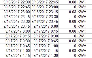 The irrigator finally remedied but this telling data trend would have caught it. The recordation value of .08 is below par and the interval is unusual. This pattern repeats many times. What is happening is that the motor is attempting an auto startup but failing in the attempt. Evidently the irrigator’s timing of his inspection rounds was such that he missed the momentary start|stop anomaly.
Irrigation Old Time: The Irrigator is practically redundant. See how much we can do from the remote office? Still, we need someone to establish the Sets. I remember when the Irrigator carried and actually used a shovel. The long handle was convenient for leaning upon 😉 Rubber [Irrigator] boots, and a cowboy hat to block the hot sun completed the look. The Irrigator made his set and watched for water that was getting away or (more hopefully) about to… It was a learned procedure — kind of like the more meaningful methods of today.
Thanksgiving
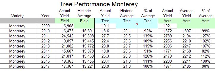
Regarde our almond tree performance this year! We had set expectations for this year’s crop knowing that quite a few of the trees went MIA during the springtime blowover. The harvest totals are nearly finalized and aside from the reduction in tree count, the trees that are still upstanding have done a superb job.
These results for our Monterey variety are fairly representative. All figures are expressed in net pounds. Observe that yield per tree held to its historical average…
 [enlargeable]
Note that some years are better than other years and the farmer will try to fathom why and how that is and try to help the trees produce consistent results. A necessary step in this task is to track the year over year results as you can see in these spreadsheet snippets.
Graphical Yield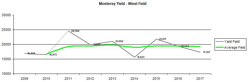 [enlargeable]
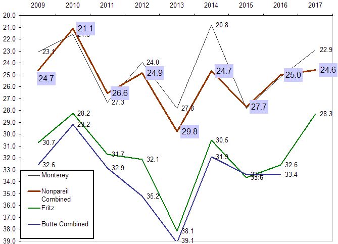
Nut sizes fluctuate as well. The nut sizing method counts the number that fit a one ounce (28.35 grams) container. Thus the smaller the size number rank then the larger the nut kernel 18 to 20 is the largest size category, 36 to 40 is the smallest. Observe the correlation between our production yield above and our nut size comparison chart that follows.
 [enlargeable]
It would seem that a prolific nut set results in smaller individual nut size and vice versa.
There is one more production metric and that one is the conversion from field harvest weight (gross) to processed meat weight (net). This is called Turnout and is derived at the Huller by dividing the net meat weight by the gross field weight.
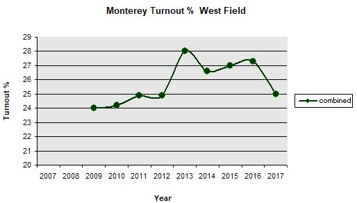
Typically, field weight yields 13 percent debris, 50 percent hulls, 14 percent shells, and 23 percent clean almond meats and pieces, but these ratios are variable as you can see. So, at 25.3% our Turnout was adequate.
The Butte will be processed soon and that will wrap things up for 2017. We have much to give thanks for.
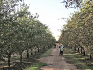
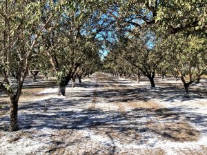
Winter Sanitation
Chemicals are used for controlling Navel Orange Worm (NOW) a pest that sometimes plagues growers, but another effective and sustainable method is sanitation. We marginalize a conducive breeding habitat by removing postharvest Mummie Nuts – a food source. Mummie shaking, either by machine or by hand using polling sticks does the trick.
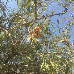
I took postharvest snapshots at our orchard last month:
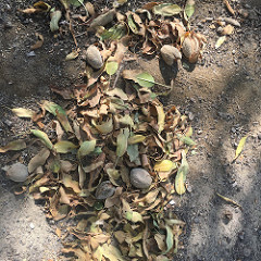
Removal is normally accomplished during winter, after rain and days of fog have weakened the nut’s attachment to the tree, allowing growers to
re-shake their trees, sweep and then grind the nuts using flail mowers. As noted in the following Blue Diamond Growers report: some are not waiting and are sending hand crews into their orchards to knock the mummies to the ground using poles. Everyone in the valley is hoping for another wet winter with ample rainfall. Unfortunately, last year’s deluge prevented quite a few from sending shakers into the orchards and after enduring the damage present in the 2017 crop, some are making extra efforts to ensure that their orchards will be free of all mummy nuts going into the 2018 growing season. The combination of over-wintering larvae coming into the 2017 crop, coupled with the high temperatures experienced in July, which prolonged the hull split resulted in extremely high NOW populations that created significant problems for growers throughout the 2017 harvest.
Luckily, our orchard has escaped excessive NOW population.
Also, the report mentions that many growers [at this time] are applying soil amendments, such as gypsum or lime to correct soil salinity and pH problems. We have ordered gypsum and compost to be spread to combat our own salinity issue at the rate of 2 tons to the acre each.
Post Harvest
This years almond crop has been picked up and now critical post-harvest irrigation, and soil amendment (fertilizer application) begin almost as soon as the nuts leave the orchard. We are mindful to see to the needs of our trees which despite environmental challenges this year performed quite well for us.
Even though relative peace and quiet have returned to the orchard, there is a continuation behind the scenes. While not directly hands on we still follow the cycle of our crop and it is interesting to know the process.
Truckloads [38] arrive at our Huller/Sheller, the Central California Almond Growers Association (CCAGA), where they are temporarily stockpiled. Just as we were careful to monitor moisture, avoid mixing 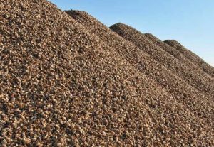 varieties, and control contamination, the huller must do the same. The product is exposed and rain and fog which will be the norm soon. In the event of early rain then plastic tarps can be used as cover but this is labor intensive and can be problematic. Their best bet is expedited processing.
This is a snippet from a CCAGA stock pile grower history print out. You can see that our Butte variety from the East Field were delivered by the truck load [4] and went into the stockpile identified as KNB74
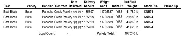
The individual loads were identified by receipt and weight certificate numbers which are all part an important chain of accounting.
What does the CCAGA do: The Huller removes the outer hull (repurposed for livestock feed) and the inner shell as well and then delivers the clean and debris free raw nut to our contracted packing company, Panoche Creek. You may have heard of the marketing brand Blue Diamond; this is a [competitive] packing house cooperative – credit the stockpile photos you see here.
Not all almond consumers like them raw by the way. Demand for nuts sold with the inner shell intact has been on the rise. They go to foreign buyers and command a premium so we are happy to furnish them inshell.
The next post will describe the processing at Panoche Creek Packing and then finally, a detailed look at the paper trail progression from end to end and how to decipher it.
Scientific Irrigation
I should think that a green thumb, who through tried and true experience — knowing the synergy between plant, sun, and water — could dig down a few inches grasp and squeeze soil in his hand, look at the plant and say needs or does not need irrigating. To obtain this cosmic sense one would have to be mentored as an apprentice and have years of hit/miss experience. Naturally the goal is to have healthy and productive growing and have more hits than misses but there is an [upward] trending motive and that is one of ecological conservation. Also, water is an expensive resource. Here is the short course using Wateright – a scientific tool from the Fresno State University. What comes first the discussion or the explanation of terminology? Feel free to skip around to get a handle on it. It is some interesting stuff if you’ve wondered (scientifically) when to irrigate and for how long. Hope you don’t find it too dry (sorry)
Disclaimer : I don’t pretend to fully comprehend the interpretation of the output from the formulae or the strategic use of moisture control for plant yield and pest control. Follows is an exercise in learning discovery. I’ve gathered definitions of terms and immersed myself in the science of irrigation using one of several scheduling tools available to farmers. My primary presentation is how soil holds water (see available water) and how plants consume water (see Transpiration).
In this 2017 Wateright Water Balance tabulation for the Section 30 Ranch, weather data from Five Points/WSFS USDA is utilized to calculate ETo (see below) . This station is part of the California Irrigation Management Information System network (CIMIS). It is a network of standardized weather stations scattered throughout California which report weather data (emphasis is sun exposure / air temperature) on an hourly basis and a reference point for evaporative demand for our micro-region.
A Water Balance FORM used data from the CIMS e.g. Potential ETc column is pre-populated. There were some constants, such as soil type, irrigation efficiency, and canopy coverage assumptions that I had to configure. Otherwise, the only daily inputs to the form by the farmer is Gross Water Applied in inches and Rain minus Runoff in inches. The tabulation output i.e all other columns are then presented in the printout follows: Wateright Moisture Balance 2017 (download link)
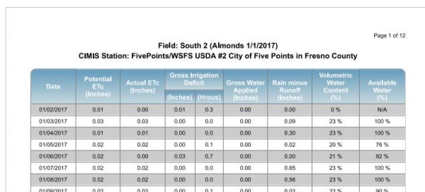
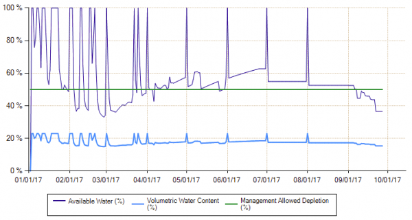
Interpretation: The farmer would like to have the actual ETc match the potential ETc for maximum plant performance. He doesn’t want to see the Volumetric Water Content go much below MAD
Explanation of Terms that will help interpret the Water Balance tool.
ET is Evapotranspiration — the process by which water is transferred from the plant leaf to the atmosphere by evaporation. for most of the growing season, the majority of the seasonal ET is from transpiration. Transpiration losses are usually high and are directly linked to plant growth and productivity. This is because the pathway for transpiration in plants is the same one that allows for plant intake of carbon dioxide. Both exchange processes occur through pores called stomates on the leaf surface. Stomates are fully open when plants receive enough water through the soil and when both transpiration and photosynthesis are occurring at maximum rates. If soil water becomes limiting, stomates begin to close causing a decrease in transpiration and photosynthesis i.e. growth production
ETo is simply a reference number which represents an estimate of evapotranspiration (ET) from an extended surface of 3 to 6 inch (8 – 15 cm) tall green grass cover of uniform height, actively growing, completely shading the ground, and not short on water. All of the CIMIS weather stations throughout the state are situated within a small grass field which is optimally irrigated. Thus, instruments attached to the weather station datalogger measure weather parameters that would directly affect ETo estimates such as solar radiation, air temperature, humidity, wind and rain. This data is incorporated within the weather station’s database and calculates a reference evapotranspiration (ETo) number every hour.
ETc is calculated by multiplying reference evapotranspiration (ETo) by the actual crop coefficient (Kc actual), ETc = ETo * Kc actual. The daily ETo values are from the CIMIS weather station, and daily actual Kc values are calculated based on dates and values entered in the ‘field setting’ multiplied by a water stress coefficient (Ks), Actual ETc = ETo * Kc * Ks.
Potential ETc is calculated by multiplying reference evapotranspiration (ETo) by the crop coefficient (Kc), ETc = ETo * Kc. It is the best case scenario for the plant to operate at 100%
Actual ETc is calculated by multiplying reference evapotranspiration (ETo) by the actual crop coefficient Kc * Ks
Kc or crop coefficient is a numerical factor that relates to the ET of an individual crop. Tall grass has a different Kc than a tree as an example. The Kc might vary through out the growing cycle e.g. as the tree canopy becomes fuller.
Ks values range from zero to one (0 to 1) and reduce the value of Kc when soil water is not adequate to sustain potential ETc. When the soil water level is above Management Allowed Depletion (MAD), Ks is equal to one, and Actual ETc = Potential ETc. When the soil water level declines below MAD, plants begin to experience water stress, Ks values are less than one, and ETc will not occur at potential rate, Actual ETc<Potential ETc. The Ks values become increasingly smaller as soil dries below MAD.
Gross applied water is equal to net applied water divided by our irrigation efficiency. We know how many acre/feet are applied in a given month but we don’t know exactly how it is proportioned (which Field). I make the assumptions that all fields receive the same amount. Convert the acre/feet (from our meter) to acre/inches and then divide the result by 220.62 acres gives the number of inches applied. Also, I don’t know what specific day the irrigation is applied; so I can only input the monthly total. That’s why is shows up on the last day of the month as a lump sum in the tabulation.
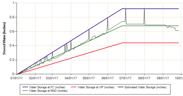
Gross irrigation deficit is the amount of water needed to bring the soil back to ‘field capacity’. It is given as depth (inches) of irrigation water and hours of running the well pumps. (Another constant I entered during tool setup. i.e. number of drip system emitters per tree and flow rate/per)
By default no runoff is assumed. Rain minus runoff is weather station data. I’ve added rainfall totals to the tabulation form using a nearby Personal Weather Station (PWS) at Kerman, CA
Available Water is the amount of water that is held by the soil between Field Capacity (FC) and Permanent Wilting Point (PWP) that crops can extract from the root zone. Water held between FC and PWP is considered to be 100% of available soil water. Soil water above FC cannot be retained and will be lost by drainage.
Not all the water between FC and PWP is Readily Available Water (RAW) to crops. When the soil water drops below a threshold value known as Management Allowed Depletion (MAD), crops begin to experience water stress and actual crop ETc falls below potential crop ETc. Moisture below PWP is strongly bonded to the soil and cannot be extracted by roots.
AW = available water
FC = field capacity
RAW = readily available water (to the plant) — MAD * AW
PWP = permanent wilting point
MAD = management allowable depletion — Default MAD value is 50%. MAD usually ranges from 40% to 60%
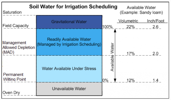 The Available Water measured in Inch/Foot refers to the holding ability of Sandy Loam. At FC this soil type can hold 2.6 inches per foot soil depth. Any greater than 2.6 inches and gravity overcomes and the excess percolates through.
So, how did our year turn out? Note that the monthly irrigation meter reading is sum totaled on the last day of the month, thus the spike in the graph below. We know how many acre/feet (from the meter)  are applied in a given month but we don’t know exactly how it is proportioned (which Field). I make the assumptions that all fields receive the same amount. Convert the acre/feet to acre/inches and then divide the result by 220.62 acres gives the number of inches applied.
Executive Summary: As a rough guideline and continuity check, generic almond trees require about 38″ of water during their growth season. We had:
- 8″ of rainfall to date
- 44 3/4″ of applied irrigation (as of 8/31)
- …for a total of 52.76″ gross applied water
On some dates the moisture content was above FC. This was primarily due to winter and early spring rainfall but was a good thing. Our fields do require periodic leaching to remove salinity and other accumulations that are naturally occurring in our aquifer sourced water.
Hmmm. It would appear that in March the irrigation got a little bit behind… Observe that the Estimated Water Storage was slightly below MAD. I’m not making a judgment. This may have been purposeful. As I say there’s much to learn!
Here’s the Dirt
The almond trees are performing as expected and our young vineyard is thriving. Soil is the foundation for plant sustainability. We can analyse it and through care and attention to the elements, maintain its balance. Moisture control, artificial and natural amendments are tools that we can use. The idea is to give back to the soil what is lost and even to enhance it when we can. This takes resources of course and to make sure that we do the right thing we need to know strengths and weakness of our ground. So, what kind of land do we have?
UC Davis and the NCRS present official USDA data in a handy survey map for our benefit:
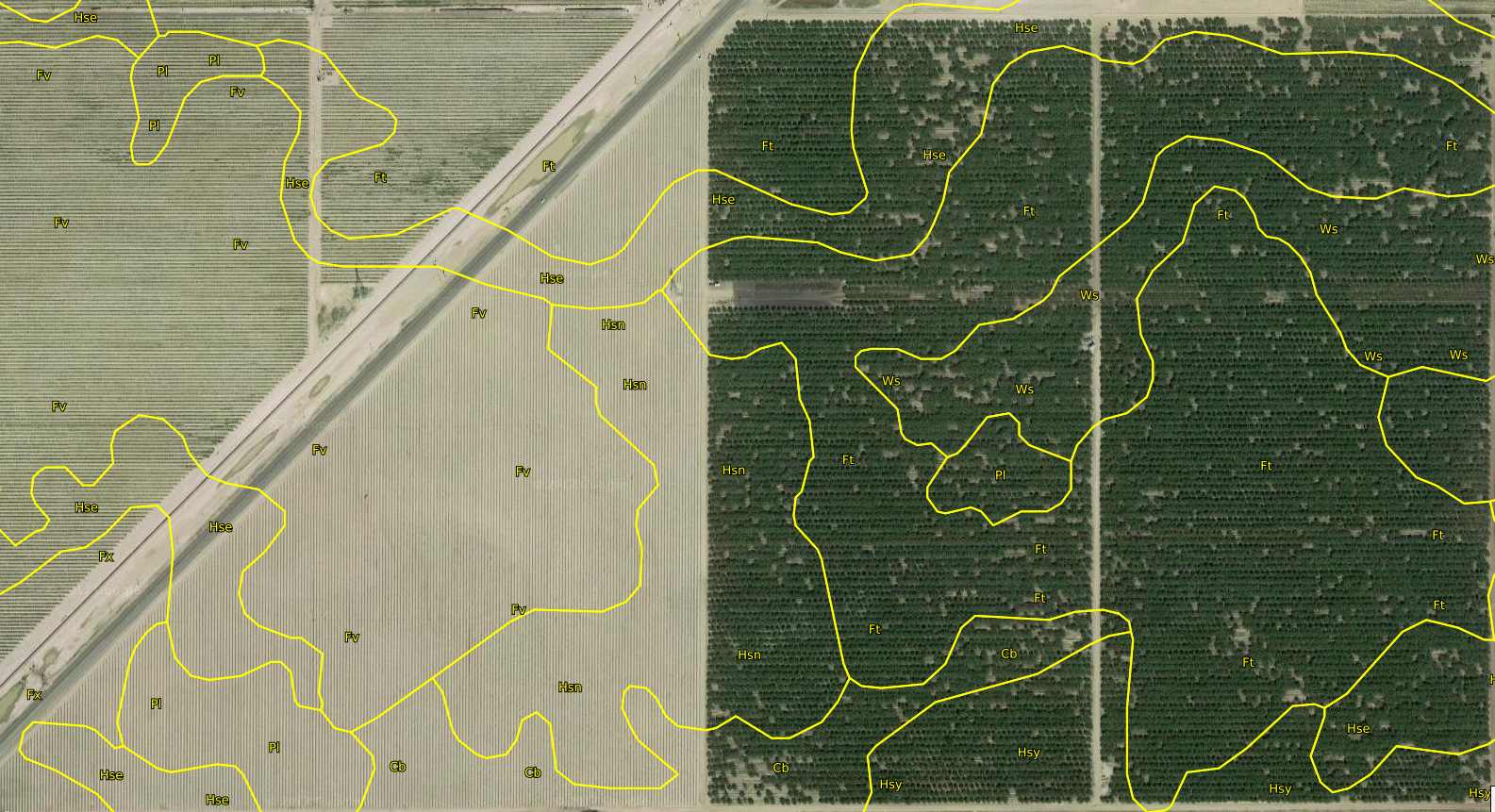
Translate the symbols from the map contour above using the legend below and you will know our soil types:
|
Symbol
|
Soil Name
|
Acres
|
Percentage
|
|
Cb
|
Cajon loamy coarse sand, saline-alkali
|
13.9
|
6.0%
|
|
Ft
|
Fresno sandy loam, shallow
|
90.0
|
38.5%
|
|
Fv
|
Fresno fine sandy loam, shallow
|
27.3
|
11.7%
|
|
Fx
|
Fresno-Traver complex
|
2.9
|
1.2%
|
|
Hse
|
Hesperia sandy loam, saline-alkali
|
28.1
|
12.0%
|
|
Hsn
|
Hesperia sandy loam, moderately deep, saline-alkali
|
29.4
|
12.6%
|
|
Hsy
|
Hesperia fine sandy loam, moderately deep, saline-alkali
|
12.8
|
5.5%
|
|
Pl
|
Playas
|
9.4
|
4.0%
|
|
Ws
|
Wunjey fine sandy loam
|
19.8
|
8.5%
|
|
Totals for Representative Mapped Area
|
233.8
|
100.0%
|
|
Each of these classes have extensive descriptions; the Fresno series for example. As a generalization you might say that our soil is sandy loam. In this part of the valley soil is naturally alkaline and low in organic matter so you could say it does need some help. Here is what it looks like when exposed by backhoe:
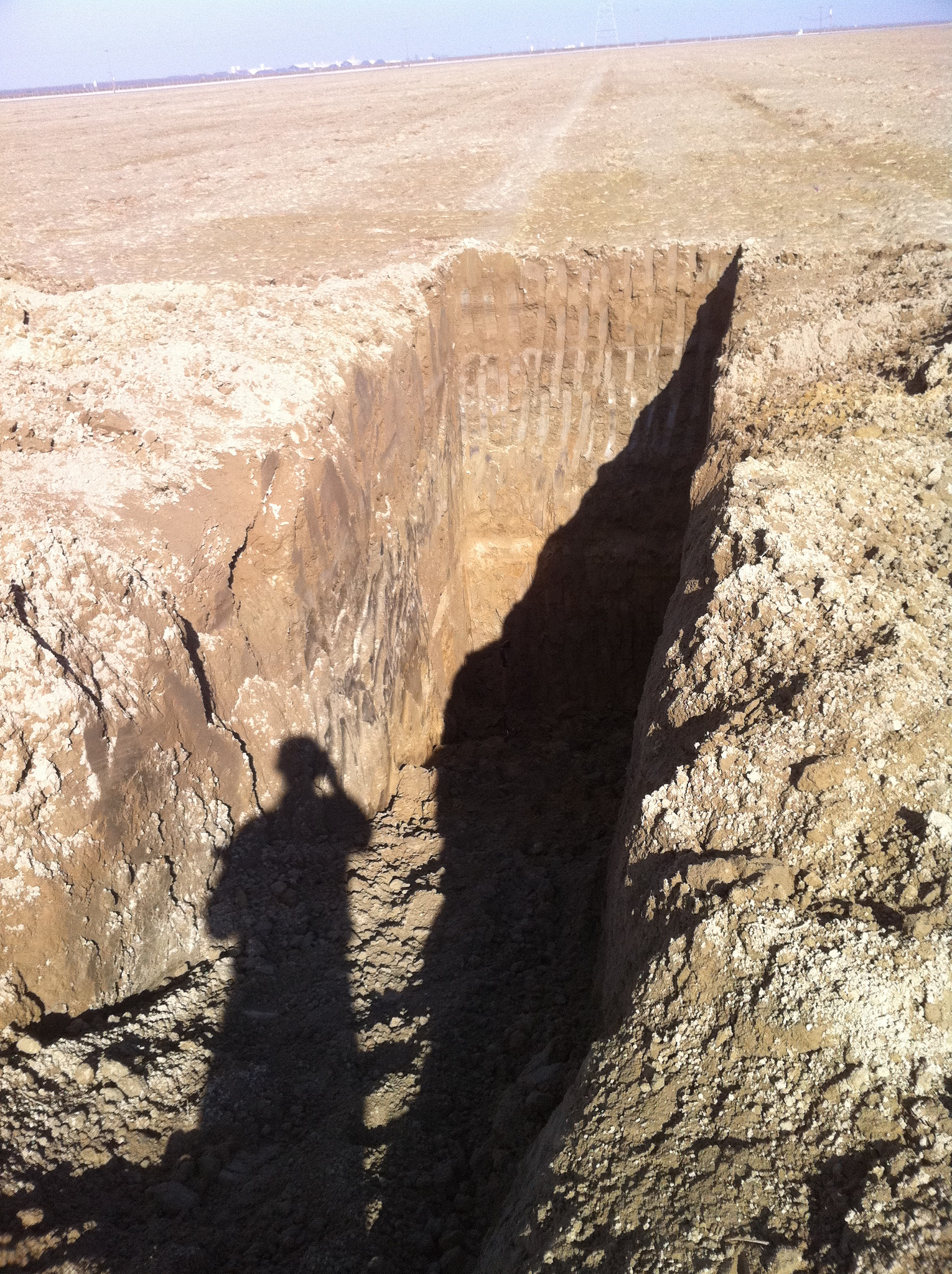
This test excavation was made when establishing our new vineyard.
The first few inches are fine sandy loam; grayish brown when moist. Next, slightly lighter colored even lower in organic material and strongly alkaline this layer has a abrupt smooth boundary. At 12-18″ we have sandy clay loam that is slightly sticky and quite firm. Just below this is strongly cemented lime silica hardpan.
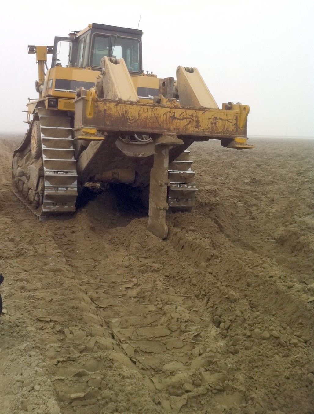
The ground trembles when this big CAT ripper sinks that 4′ shank.
Breaking up the hardpan is an elementary step. Gypsum can be employed to help resist the formulation of hardpan. Also, Gypsum will exchange calcium for sodium, releasing the sodium into solution allowing it to leach out into 24″ to 60″ stratified loam that becomes friable and less calcareous with depth .
Since we have low & medium levels of free lime we apply Sulfur to the soil profile. Soil sulfur will combine with the water and oxygen therein to form sulfuric acid taking the soil pH toward the acidic. To supplement organic material we add Compost.
Take care of your land and it will take care of you.
Minding the Till
There’s an Almond (or Wine Grape) harvest documentation chain of custody from the Weighmaster to the Processer. However, there is a leap of faith gap between the harvest collection and a transport’s first stop at the scales. In previous times we relied solely on the moral integrity of the trucker until we came to the realization that this was a security hole in our method system. What if a load (or more) were never to arrive at the Weigh Station, diverting instead? An unaccounted for trailer load would be a small skim of our grand total and would certainly line the pocket of the thief. Would we be the wiser?
It’s the modern day equivalent of horse thieving or cattle rustling. It’s a crime that’s difficult to guard against and discoverable only after the fact, if that. Commodity theft is not a fluke:
- Farm Felons Pick Off California Crops – New York Times
- In California, a New Breed of Rustlers Goes for the Nuts – NBC
- Rustlers forget about cattle and turn to nuts – San Jose Mercury
Ideally, one of us should be camping onsite to observe and document the coming and goings of all trucks with trailers. Perhaps, strategic placement of security cameras to record truck IDs or trailer license plate numbers would be smart.  As it is today, we now rely on a ranch management employee assigned the recording task. Clipboard in hand he dutifully logs the heavily loaded trailers that leave our private dirt road and hit the public highway. Or, does he… Could he be in cahoots for part of a cut? We rely upon our monitor’s diligence and have faith in his honesty. Small need for conspiracy paranoia — but a topic to be aware of and to consider.