I should think that a green thumb, who through tried and true experience — knowing the synergy between plant, sun, and water — could dig down a few inches grasp and squeeze soil in his hand, look at the plant and say needs or does not need irrigating. To obtain this cosmic sense one would have to be mentored as an apprentice and have years of hit/miss experience. Naturally the goal is to have healthy and productive growing and have more hits than misses but there is an [upward] trending motive and that is one of ecological conservation. Also, water is an expensive resource. Here is the short course using Wateright – a scientific tool from the Fresno State University. What comes first the discussion or the explanation of terminology? Feel free to skip around to get a handle on it. It is some interesting stuff if you’ve wondered (scientifically) when to irrigate and for how long. Hope you don’t find it too dry (sorry)
Disclaimer : I don’t pretend to fully comprehend the interpretation of the output from the formulae or the strategic use of moisture control for plant yield and pest control. Follows is an exercise in learning discovery. I’ve gathered definitions of terms and immersed myself in the science of irrigation using one of several scheduling tools available to farmers. My primary presentation is how soil holds water (see available water) and how plants consume water (see Transpiration).
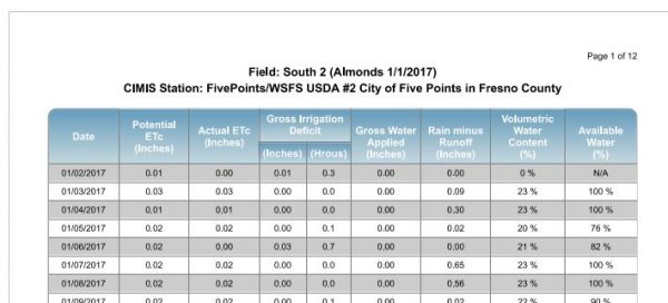
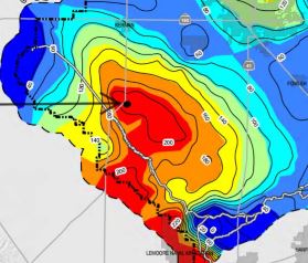
In this 2017 Wateright Water Balance tabulation for the Section 30 Ranch, weather data from Five Points/WSFS USDA is utilized to calculate ETo (see below) . This station is part of the California Irrigation Management Information System network (CIMIS). It is a network of standardized weather stations scattered throughout California which report weather data (emphasis is sun exposure / air temperature) on an hourly basis and a reference point for evaporative demand for our micro-region.
A Water Balance FORM used data from the CIMS e.g. Potential ETc column is pre-populated. There were some constants, such as soil type, irrigation efficiency, and canopy coverage assumptions that I had to configure. Otherwise, the only daily inputs to the form by the farmer is Gross Water Applied in inches and Rain minus Runoff in inches. The tabulation output i.e all other columns are then presented in the printout follows: Wateright Moisture Balance 2017 (download link)
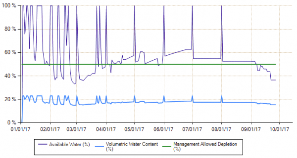
Interpretation: The farmer would like to have the actual ETc match the potential ETc for maximum plant performance. He doesn’t want to see the Volumetric Water Content go much below MAD
Explanation of Terms that will help interpret the Water Balance tool.
ET is Evapotranspiration — the process by which water is transferred from the plant leaf to the atmosphere by evaporation. for most of the growing season, the majority of the seasonal ET is from transpiration. Transpiration losses are usually high and are directly linked to plant growth and productivity. This is because the pathway for transpiration in plants is the same one that allows for plant intake of carbon dioxide. Both exchange processes occur through pores called stomates on the leaf surface. Stomates are fully open when plants receive enough water through the soil and when both transpiration and photosynthesis are occurring at maximum rates. If soil water becomes limiting, stomates begin to close causing a decrease in transpiration and photosynthesis i.e. growth production
ETo is simply a reference number which represents an estimate of evapotranspiration (ET) from an extended surface of 3 to 6 inch (8 – 15 cm) tall green grass cover of uniform height, actively growing, completely shading the ground, and not short on water. All of the CIMIS weather stations throughout the state are situated within a small grass field which is optimally irrigated. Thus, instruments attached to the weather station datalogger measure weather parameters that would directly affect ETo estimates such as solar radiation, air temperature, humidity, wind and rain. This data is incorporated within the weather station’s database and calculates a reference evapotranspiration (ETo) number every hour.
ETc is calculated by multiplying reference evapotranspiration (ETo) by the actual crop coefficient (Kc actual), ETc = ETo * Kc actual. The daily ETo values are from the CIMIS weather station, and daily actual Kc values are calculated based on dates and values entered in the ‘field setting’ multiplied by a water stress coefficient (Ks), Actual ETc = ETo * Kc * Ks.
Potential ETc is calculated by multiplying reference evapotranspiration (ETo) by the crop coefficient (Kc), ETc = ETo * Kc. It is the best case scenario for the plant to operate at 100%
Actual ETc is calculated by multiplying reference evapotranspiration (ETo) by the actual crop coefficient Kc * Ks
Kc or crop coefficient is a numerical factor that relates to the ET of an individual crop. Tall grass has a different Kc than a tree as an example. The Kc might vary through out the growing cycle e.g. as the tree canopy becomes fuller.
Ks values range from zero to one (0 to 1) and reduce the value of Kc when soil water is not adequate to sustain potential ETc. When the soil water level is above Management Allowed Depletion (MAD), Ks is equal to one, and Actual ETc = Potential ETc. When the soil water level declines below MAD, plants begin to experience water stress, Ks values are less than one, and ETc will not occur at potential rate, Actual ETc<Potential ETc. The Ks values become increasingly smaller as soil dries below MAD.
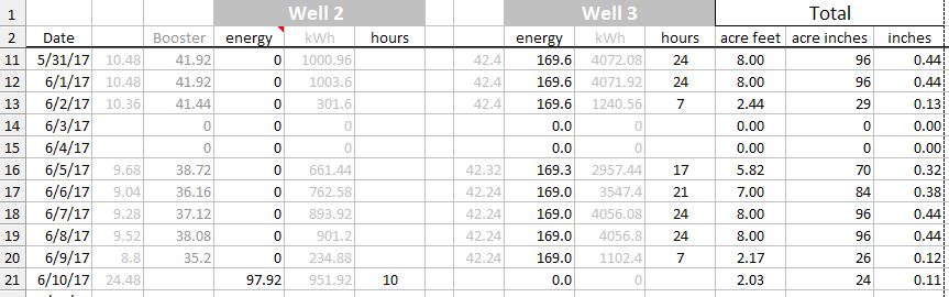
Gross applied water is equal to net applied water divided by our irrigation efficiency. We know how many acre/feet are applied in a given month but we don’t know exactly how it is proportioned (which Field). I make the assumptions that all fields receive the same amount. Convert the acre/feet (from our meter) to acre/inches and then divide the result by 220.62 acres gives the number of inches applied. Also, I don’t know what specific day the irrigation is applied; so I can only input the monthly total. That’s why is shows up on the last day of the month as a lump sum in the tabulation.
Gross irrigation deficit is the amount of water needed to bring the soil back to ‘field capacity’. It is given as depth (inches) of irrigation water and hours of running the well pumps. (Another constant I entered during tool setup. i.e. number of drip system emitters per tree and flow rate/per)
By default no runoff is assumed. Rain minus runoff is weather station data. I’ve added rainfall totals to the tabulation form using a nearby Personal Weather Station (PWS) at Kerman, CA
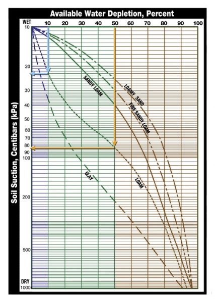
Available Water is the amount of water that is held by the soil between Field Capacity (FC) and Permanent Wilting Point (PWP) that crops can extract from the root zone. Water held between FC and PWP is considered to be 100% of available soil water. Soil water above FC cannot be retained and will be lost by drainage.
Not all the water between FC and PWP is Readily Available Water (RAW) to crops. When the soil water drops below a threshold value known as Management Allowed Depletion (MAD), crops begin to experience water stress and actual crop ETc falls below potential crop ETc. Moisture below PWP is strongly bonded to the soil and cannot be extracted by roots.
AW = available water
FC = field capacity
RAW = readily available water (to the plant) — MAD * AW
PWP = permanent wilting point
MAD = management allowable depletion — Default MAD value is 50%. MAD usually ranges from 40% to 60%
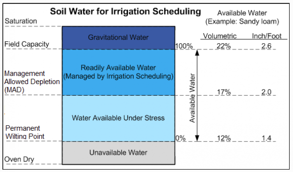 The Available Water measured in Inch/Foot refers to the holding ability of Sandy Loam. At FC this soil type can hold 2.6 inches per foot soil depth. Any greater than 2.6 inches and gravity overcomes and the excess percolates through.
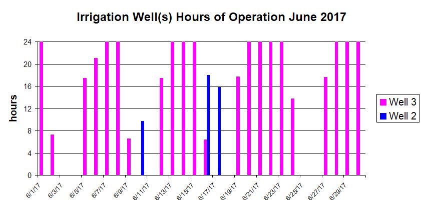
So, how did our year turn out? Note that the monthly irrigation meter reading is sum totaled on the last day of the month, thus the spike in the graph below. We know how many acre/feet (from the meter) 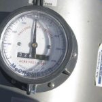 are applied in a given month but we don’t know exactly how it is proportioned (which Field). I make the assumptions that all fields receive the same amount. Convert the acre/feet to acre/inches and then divide the result by 220.62 acres gives the number of inches applied.
Executive Summary: As a rough guideline and continuity check, generic almond trees require about 38″ of water during their growth season. We had:
- 8″ of rainfall to date
- 44 3/4″ of applied irrigation (as of 8/31)
- …for a total of 52.76″ gross applied water
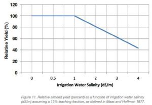
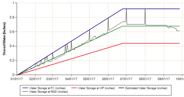
On some dates the moisture content was above FC. This was primarily due to winter and early spring rainfall but was a good thing. Our fields do require periodic leaching to remove salinity and other accumulations that are naturally occurring in our aquifer sourced water.
Hmmm. It would appear that in March the irrigation got a little bit behind… Observe that the Estimated Water Storage was slightly below MAD. I’m not making a judgment. This may have been purposeful. As I say there’s much to learn!
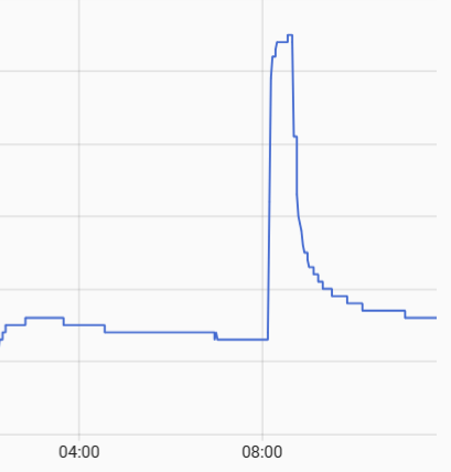
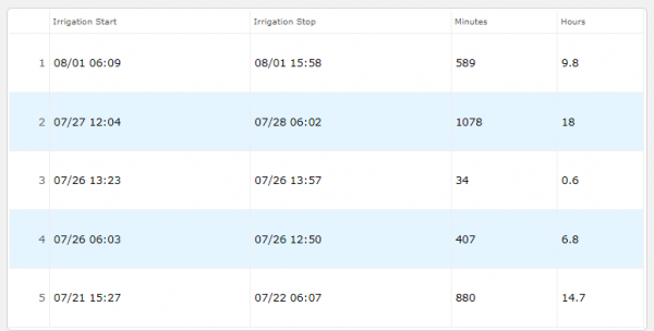
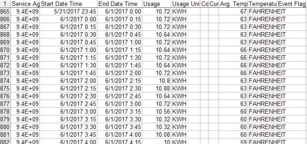
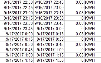 The irrigator finally remedied but this telling data trend would have caught it. The recordation value of .08 is below par and the interval is unusual. This pattern repeats many times. What is happening is that the motor is attempting an auto startup but failing in the attempt.
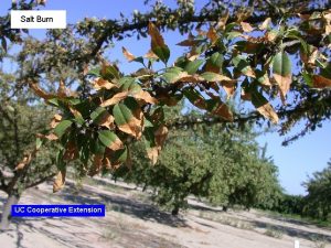
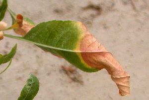 … not to be confused with